The review of fourteen fatigue models is presented in [34] with an emphasis on summarizing the features and applications of each fatigue model. The models are classified into five categories: stress-based, plastic strain based, creep strain-based, energy-based and damage-based methodology. The stress-based classification is based on the application of a force or stress to a component causing a resulting strain. Typically, stress-based fatigue applies to vibrational or physically shocked or stress component. In the strain-based fatigue models a strain is applied, resulting in stresses within a component. The types of strain-introduced fatigue further can be divided into two groups, namely plastic strain or creep strain. Plastic strain deformation focuses on the time-independent plastic effects. while creep strain accounts for the time-dependent effects. The energy-based is the newest models in use today, and are based on calculating the overall stress-strain hysteresis energy of the system. Damage-based fatigue models are based on calculating the accumulated damage caused by crack propagation and developed based on a fracture mechanics approach.
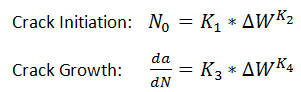
The fatigue life prediction implemented in OptiY relates most on the theoretical and experimental work of Darveaux [30-33]. It is the energy-base fatigue models and forms the largest group of models. These models are used to predict fatigue failure based on a hysteresis energy term of type of volume-weighted average stress-strain history. Fatigue energy is typically calculated using some correlation to the energy under the stress-strain hysteresis loop. The model utilizes finite element analysis to calculate the inelastic strain energy density ΔW accumulated per cycle during a thermal or mechanical cycle load. The strain energy density is then used with crack growth data to calculate the number of cycles to initiate cracks and the number of cycles to propagate cracks. It was shown in [35] that the crack growth data were fit to relations of forms:
where N is the number of cycles, N0 is the number of cycles to initiate the cracks, K1 is the crack initiation factor, K2 the crack initiation exponent, a is the crack length, K3 is the crack growth factor and K4 is the crack growth exponent. These parameters are dependent on FEA-model and material properties, and they have to be validated by experimental data. The units of these parameters have to be set appropriate to each other to get correct fatigue results.
To predict fatigue life from crack growth data, one needs to assume a certain failure distribution. Clech [35] has shown that a 3-parameter Weibull distribution is most appropriate. The cumulative distribution of failures F for this Weibull distribution is given by:

Where N is the number of cycles, Nff is the failure free life, αw is the characteristic life at which 63.2% of the population has failed, and βw is the shape factor which indicates the amount of the scatter in the data.
Since the crack growth rate was shown to be constant during thermal or mechanical cycling, the fatigue life can be calculated by adding the number of cycles for crack initiation plus the number of cycles to growth the cracks across the total crack length. The characteristic life is given by:
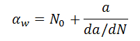
where "a" is the total crack length. It was shown in [30] that the maximum crack length in the population was approximately 2X the characteristic length. Hence it would be expected the failure free life to be approximately one half of the characteristic life:
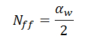
In practice, one does not test an infinitively large sample size, so the number of cycles to first failure will be greater than the failure free life. The cycles to first failure is given by:
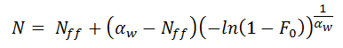
where F0 is the calculated in terms of median rank:
where Ss is the sample size.
A comment should be made about relative and absolute predictions. In most cases, there is at least one data set of measured fatigue life for a product. In this scenario, relative predictions can be made. The procedure is to first calculate life for the known case (measured data), then calculate life the unknown cases. A relative life prediction can be made from these two calculations.
For the case where the product is only in the concept stage, and there is no measured data available, absolute prediction can be made. Also, if one is comparing measured versus predicted results for a wide range of product types, material sets and test conditions, the prediction is more of absolute nature. For absolute predictions, the accuracy is somewhat less, but typically +/- 2X or better. If one does a very good job at characterizing the material properties and modeling the exact configuration that was tested, the accuracy can be better than +/-2X.