Gaussian Process
1. Gaussian Process Regression
The Gaussian process,
well-known as Kriging, is multivariate normal distributions with finite
dimensionality [14, 25-27]. The Gaussian process model is composed of a global
model f(x) and the stochastic Gaussian process Z(x)
presenting a deviation from the global model:
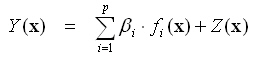
Where f(x) the
polynomial regression function with regression coefficients β, and Z(x) is a stationary
stochastic Gaussian process N(0, K) having zero mean and covariance
function K. x is an m-dimensional vector of input parameters.
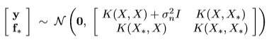
For the stochastic process
Z(x), suppose that the training data consists of the computer
output y at the input data X = {x1, x2,
.., xn} and that f* is the being predicted at x*.
The Gaussian process model has got the multivariate normal distribution:
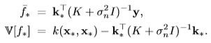
Therefore, the prediction
for f* is the mean of the multivariate normal distribution and its variance
V(f*) is the uncertainty of the prediction:
1.1
Covariance Functions
Covariance function (K=R) is the crucial ingredient in a Gaussian process predictor, as it encodes the assumptions about the interpolation function between x1 and x2. Therefore, different famos stationary covariance functions [27] have been implemented:
· Square Exponential
· Exponential
· Gamma-Exponential
· Matern Class 3/2
· Matern Class 5/2
· Periodic
· Rational Quadratic
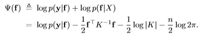
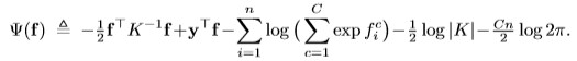
where w, λ and α are hyper-parameters, which have to be found
using optimization procedure to maximize the likelihood function of the
multivariate normal distribution:

1.2 Adaptive Gaussian Process
The Gaussian process
returns not only the prediction value, also the uncertainty of the prediction
for the regression function. Thus, the confidence interval is available over
all the regression function space. That leads to an efficient way called
adaptive Gaussian process making the regression function more accurately with
few number of data points. The adaptive Gaussian process is an iterative
process. For the initial data points, the initial Gaussian process will be
generated. Based on the calculated uncertainties, the data point on the
parameter space returning the maximal uncertainty will be sampled for the next
generating of the Gaussin process. This adaptive
process will be iterative carried out until the maximal uncertainty the
user-defined limit or a number of sampled data points have been obtained.
2. Gaussian Process
Classification
The regression is
considered, when the output is continuous real value. Classification is another
important problem, where the output is the discrete value, states or classes
[60-76]. While regression represents the analog simulation, classification
deals with digital simulation, the output is assigned to one of C classes (C
>1). for Gaussian process classification, the
latent f(x) function is introduced. The input data x
is approximated by this latent function using Gaussian process regression with
Laplace approximation. Then, the latent function f will be squash through a
function to obtain probability π assigning to one of the classes C .
We decide 2 cases, binary classification (C=2) and multiple classification
(C>2)
2.1 Binary Classification
Laplace method utilizes a
Gaussian approximation to the posterior with the latent fuction
f:
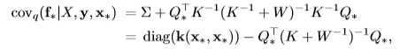
The posterior mean for f uner the Laplace approximation can be expressed:
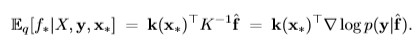
and the variance of the prediction is:

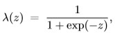
The latent function f will
be squash to one of the binary class using the regression function:
2.2 Multiple Classification
The posterior for the multple classification problem is more complex.
Thus, the posterior mean
for f is bellow:

and the variance of the prediction:
The latent function f is
assigned to one of C class using the soft-max function:
3. Sparse Gaussian Process by Low-Rank Approximation
The representing for the input data X = {x1, x2, .., xn} is the covariance matrix K with n descending ranks: λ1, λ2,...,λr , .. , λn . If the number of the input data is extremely huge, the computing of the Gaussian process based matrix operations is very expensive. The matrix approximation is an efficient way to reduce the input data to a low-rank matrix with (r < n) for cheaper computing and less quality loss. The small ranks of the covariance matrix (r+1, r+1, ... n) will be cut off. The approximated matrix will have got only r ranks, but represents the initial covariance matrix with minimal differences. This process is called sparse Gaussian process.