Hilbert Space

Hilbert spaces provide a user-friendly framework for studying infinite-dimensional phenomena, such as functional analysis, quantum mechanics, and many areas of mathematics and physics. It is a complete inner product space, which is a vector space equipped with an inner product that satisfies certain properties [88-91, 100]. Let's break down the key components of a Hilbert space:

1. Feature space or vector space is a collection of objects called vectors that can be added together and multiplied by scalars. In the context of a Hilbert space, these vectors are typically functions or sequences, although they can represent other mathematical objects as well.
2. An inner product is a mathematical operation that takes two vectors and returns a scalar. It satisfies several properties, including linearity, symmetry, and positive-definiteness. The inner product is often denoted by <x, y> and can be thought of as a measure of the similarity or "angle" between the two vectors.
3. Completeness is a crucial property of a Hilbert space. It means that every Cauchy sequence in the space converges to a limit that is also in the space. In other words, there are no "missing" points or "gaps" in the space, and any sequence of vectors that gets arbitrarily close to each other has a well-defined limit.

Hilbert spaces have rich mathematical structures, two standard components for vector spaces are implemented in OptiY:

• Polynomial vector space:
• Dirichlet vector space:

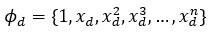
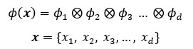
Where n is the dimension of the vector space, which can be infinite. The Hilbert space of d-dimension is the inner product of these feature spaces:

Given are m input data vectors {x1, x2, … ,xm} and the output point {y1, y2, …, ym}. The Hilbert space represents thus the input matrix ϕ = {ϕ(x1), ϕ(x2), …, ϕ(xm)} and the output vector y = {y1, y2, .., ym}. The optimization problem by machine learning for classification and regression is formulated as following:

where β are coefficients of Cauchy sequences being optimized. There are two general following methods for solving this optimization problem.

Kernel Method (RKHS)

This method is well-known as Reproducing Kernel Hilbert Space (RKHS) [91]. A reproducing kernel is a symmetric function k

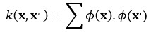
which produces a positive semi-definite matrix K by m data points

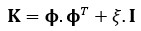
Where ξ the Gaussian noise and I the unity matrix. The optimization problem is now formulated as minimization the negative marginal likelihood as the Gaussian process:

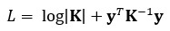
the coefficients are calculated as following

The covariance functions of Gaussian process can be formulated as Hilbert space via Fourier-transformation:

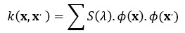
Where S is the spectral density with the frequency λ of the Fourier series for the corresponding covariance function of the Gaussian process.

The advantage of this method is the accuracy of the solution, but it requires a lot of memory for matrix calculation. The method is useable only for linear partial differential equations.

Nonlinear Method (Neural Networks)

By this method, the Hilbert space is considered as nonlinear regression as neural networks. The weights of this networks are the coefficients β of the Cauchy sequences. The Loss function being minimized is defined for single data point I as:

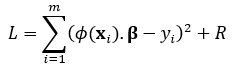
Where R is the regularization term for the coefficients β, which can be L1 or L2.

The advantage of this method is that the stochastic gradient descent method can be used finding the coefficients. Thus, big data can be optimized with less memory and fast. The method is useable also for nonlinear partial differential equations.