The method of least squares, also known as regression analysis, is used to model numerical data obtained from observations by adjusting the parameters of a model so as to get an optimal fit of the data. The best fit is characterized by the sum of squared residuals have its least value, a residual being the difference between an observed value and the value given by the model.
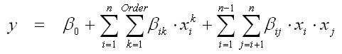
The used approximation function of the linear regression analysis is the polynomial series in any order:
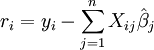
The first objective of regression analysis is to best-fit the data by adjusting the parameters of the model. Of the different criteria that can be used to define what constitutes a best fit, the least squares criterion is a very powerful one. The objective function, S, is defined as a sum of squared residuals ri
![]()
where each residual is the difference between the observed value and the value calculated by the model:
The best fit is obtained when S, the sum of squared residuals, is minimized. Subject to certain conditions, the parameters then have minimum variance and may also represent a maximum likelihood solution to the optimization problem. From the theory of linear least squares, the parameter estimators are found by solving the normal equations:
![]()
In matrix notation, these equations are written as:
![]()
The parameters β is calculated by solving the linear matrix equations:
![]()
The required model calculations result from the number of stochastic variables n and the polynomial order O
(n2-n)/2 + O*n +1
Regularization is the method to avoid overfitting by least square. The regularization is formulated as the minimization problem:
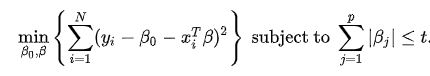
This problem is solved by the low-rank approximation of the input matrix XTX. This matrix has got n descending ranks λ1, λ2,... λn, where λ1 is the max rank. The rank is irreciprocal to the coefficient β. Therefore, if all small ranks (λ < percent * λ1) are removed from the matrix, the corresponding large coefficient β will be zero. Thus, the low-rank apprximation regularies the overfitting of the least square method.