Stochastic Settings

Click the stochastic item in the explorer to edit its options in the property window. The name, unit and comment of the stochastic parameter can usally be changed here. As alternative for editing of a large number of stochastic design parameters, the stochastic editor can be used.

• Design of Experiment

  These Parameters are used for design of experiment, which are calculated by the original model .

• Nominal

  This is the nominal value of the stochastic distribution. It represents the mean value and within the location of the distribution. If  a nominal parameter and a stochastic parameter is assigned to the same model parameter, the total nominal value for this model parameter is the sum of both nominal values.

   

• Tolerance

  This is the range of the probability distribution, whose mean value is the nominal value above. The  tolerance value is used to fix upper and lower boundaries for sampling and it represents also the variance of the distribution.

   

• Accuracy

  This is the accuracy for the sampling point from the tolerance value. Thus, user can specify the type of the parameter value return to the simulation model . The accuracy must be positive or zero:

• Accuracy = 0    ->  parameter value = real

• Accuracy = 1    ->  parameter value = integer

• Accuracy = 0.2 ->  parameter value = a multiple of 0.2 (increment = 0.2)

• Value List

  if the type of the parameter is discrete (Type = Discrete), user can specify the value list for this parameter, Only the value from this list can be assigned to this parameter. 

   

• Distribution

  This is the distribution type for this stochastic parameter. There are 3 types of distribution: Normal Distribution, Uniform Distribution and the generalized  Lambda Distribution. If the option "Distribution = Lambda Distribution", the lambda parameters of the generalized lambda distribution can be changed to fit to a required distribution. But it is too difficult to get the correct lambda values. Therefore, central moments are used to fitt the required distribution:

• Skewness

  It is a measure of the asymmetry for the probability distribution. All symmetric distributions have skewness of zero.

• Kurtosis

  It is a measure of the peakedness for the probability distribution. Lower kurtosis means more of the variance is due to infrequent extreme deviations, as opposed to frequent modestly-sized deviations. A normal distribution has got the kurtosis of 3.

• Show Graphics

  The lambda distribution can shown graphically for better setting. The graphic window will automatically be updated, if the nominal, tolerance, skewness and kurtosis are changed. The upper and lower boundaries of tolerance range, which are defined by the tolerance value (+- Tolerance/2), are displayed with 2 red lines. The mean value of the distribution is characterized also by a red line.

• Distribution Fitting

  Show the dialog fitting the stochastic distribution from measurement or manufacturing data.

• Type

  User can define the type for this parameter Constant, Random, Variable or Discrete. If the type is Constant, the parameter is fixed. By Random, the parameter is defined as random variable with tolerance value and its accuracy. The parameter value will be generated by sampling strategies inside of the tolerance value with its distribution. by Discrete, the parameter value can be only one of the values from this value list. If the parameter type is Variable, the nominal value can be changed by nominal optimization. User can set the lower and upper boundaries as well as the start step for this optimization

   

• Start Step

  This item will be only visible if the option "Start Step= Manual" is used in the optimization settings. If the option is set to "Standard", the start step for each design parameter is automatically set to 1/1000 of the defined search range by the Hooke-Jeeves-method or to 1/100 by the evolutionary algorithms.

   

• Lower Boundary

  Lower boundary is the most small value of the design parameter, which can be accepted by a nominal optimization process (Nominal Value >= Lower Boundary). If there is no lower boundary for this design parameter, set the value of the lower boundary to an extreme value (e.g. -1E100), which can be never reached by an optimization.

   

• Upper Boundary

  Upper boundary is the largest value of the design parameter, which can be accepted by the nominal optimization process (Nominal  Value ≤ Upper Boundary). If there is no lower boundary for this design parameter, set the value of the upper boundary to an extreme value (e.g. 1E100), which can be never reached by an optimization.

• Virtual Design

  This is the basics for virtual design, which calculatuions base on the fast meta model.

• Design Parameter

  The option is used, if this stochastic parameter is the design parameter or noise parameter. If it set to True, the virtual Nominal will be defined as design parameter and can be changed by the virtual optimization (e.g. Robust Design). If it is set to False, the stochastic parameter will be considered as noise or environment factor. It is fix value in the reality and must be involved in the design process.

   

• Nominal

  This is the virtual nominal value of the stochastic parameter. It used to compute the response surface based on the meta model in the section diagram. This is also the mean value of the probability distribution for this stochastic parameter, which is used to sample the output distributions using the virtual sample size.

   

• Tolerance

  This is the virtual tolerance range of the stochastic parameter. It used to compute the probabilistic variables based on the meta model. This is the range of the probability distribution for this stochastic parameter, which is used to sample the output distributions using the virtual sample size.

   

• Distribution

  This is the distribution type for virtual design. There are 3 types of distribution: Normal Distribution, Uniform Distribution and the generalized  Lambda Distribution. The parameters for lambda distribution are the same as above.

   

• Type

  It supports three types of stochastic parameter for virtual design:

• Constant

  The tolerance value of the stochastic parameter is constant. It cannot be changed.

• Variable

  The tolerance value is a optimization variable and can be changed by the optimization method. The changing increment is given by the option Accuracy.

• Discrete

  The values of tolerance can be a value of the list, which can be input by user by clicking on the option Value List..

• Lower Boundary

  Lower is the most small value of the tolerance value which can be accepted by the optimization process:

  Tolerance ≥ Lower Boundary

  At the optimization process, the tolerance value can violate the lower boundary. In this case, a penalty function will be created and handled with the highest priority to constrain the search process into the defined range. If there is no lower boundary for this design parameter, set the value of the lower boundary to an extreme value (e.g. -1E100), which can be never reached by an optimization.

• Upper Boundary

  Upper is the largest value of the tolerance which can be accepted by the optimization process:

  Tolerance ≤ Upper Boundary

  At the optimization process, the tolerance value can violate the upper boundary. In this case, a penalty function will be created and handled with the highest priority to constrain the search process into the defined range. If there is no upper boundary for this design parameter, set the value of the upper boundary to an extreme value (e.g. 1E100), which can be never reached by an optimization.

• Accuracy

  For the optimization, it is sometimes necessary to limit the accuracy of the optimization variables to satisfy the design requirements. The accuracy is the most small changing value of the optimization variable, which can be set at the optimization. The optimization step is a multiple of the accuracy. The accuracy must be positive or zero. If zero, optimization variables may be a arbitrary real value. E.g.

• Accuracy = 0    ->  tolerance value = arbitrary real value

• Accuracy = 1    ->  tolerance value = integer value

• Accuracy = 0.2 ->  tolerance value = a multiple of 0.2 (increment = 0.2)

• Cost Factor

  For the tolerance-cost optimization, several costs are caused by several tolerances. For each tolerance, a cost factor has to be defined. Higher cost factor influences more on the cost function. All cost factors are normally set standard to 1.

• Fatigue Life Prediction

This property will be only visible, if there is at least one node Strain Energy Density in the experiment. The load function can be defined for the fatigue life prediction using the meta model.

• Load Variable

  If it is True, this stochastic design parameter will be used as load function for fatigue life prediction. The field "Load Function" will be displayed in the property windows. If it is False, the stochastic design parameter is only a fix virtual nominal value for the fatigue life prediction.

   

• Load Function

  If the "Load Variable" is set to True, this field will be activated. By clicking  the field, a button will be displayed on the right side. Click the button to open a dialog for design of the load function.

  Editor: the load function can defined here using the programming language Visual Basic.NET. It is the dynamical cycle load function in time expressed by the mathematical function: Load = f(Time). The variables "Load" and "Time" are predefined and can be used without declaration. The axis "Time" with its step for a load cycle is setup in Fatigue Life Prediction Settings.

  

   

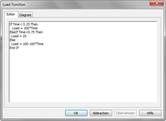
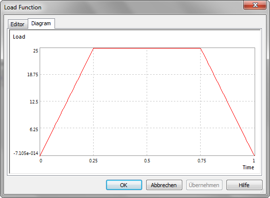
  Diagram: If the load function is defined in the editor, the graphical diagram of the dynamical load function will be shown here for checking. If there is any error of the given load function with Visual Basic, it will be displayed and the diagram will be empty. Within, the correctness of the load function can be checked.